

If you’ve made it this far, you probably want to freeze a row or a column in Excel so you don’t lose sight of the headers while scrolling through a large worksheet. It’s one of those small features that completely changes how you read a table—especially when the file starts to feel more like a dashboard than a regular spreadsheet.
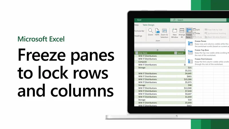
In Excel, freezing panes means locking a specific area of the sheet so it stays visible as you scroll. This lets you keep the top row, the first column, or a continuous block of rows or columns in view. The feature is available under the View tab, inside the Freeze Panes menu, and you can undo it at any time.
How to freeze the top row or the first column
The fastest way is to use Excel’s built-in quick options. Just open your file, go to View, and click Freeze Panes. In that menu you’ll see two instant actions: Freeze Top Row and Freeze First Column. You don’t need to select anything beforehand, which is exactly why it’s the most convenient route when you only want to keep the basic headers visible.
This is especially useful on sheets with lots of rows, where losing track of which column is which happens almost immediately. It also makes sense in documents where the first column acts as an index, a name field, or an identifier. Who hasn’t scrolled down hundreds of rows and ended up staring at orphaned numbers, as if Excel had decided to switch on roguelike mode?
Although Excel separates these options to save you clicks, in practice the behavior is the same as manual freezing: it creates a fixed pane that stays on screen while you move through the rest of the document.
How to freeze multiple rows or columns in Excel
When you need more than the first row or the first column, the process changes slightly, but it’s still straightforward. Select the row directly below the rows you want to freeze, or the column to the right of the columns you want to keep visible. Then go back to View, open Freeze Panes, and choose Freeze Panes again.
That selection detail is key. Excel doesn’t ask you to highlight what you want to freeze directly, but rather the point where scrolling should begin. If you click the row number or the column letter, the selection will be faster and more precise.
It’s worth keeping one important limitation in mind: you can only freeze one continuous section at a time. In other words, you can’t freeze multiple separate areas or create independent combinations within the same document. If you want to change the frozen area, you’ll have to unfreeze the previous one first. Excel is still very Excel here: powerful, yes, but with fairly strict rules.
For those who prefer keyboard-driven workflows, there’s also a shortcut to freeze panes. After selecting the appropriate row or column, press Alt + W + F + F in sequence. And if what you want is to unfreeze the view, use Alt + W + F + U.

How to unfreeze panes
If at any point you need to go back to the normal view, it’s a direct path. Open the Excel sheet, go to View, click Freeze Panes, and select Unfreeze Panes. That removes any frozen rows or columns currently on screen.
This step is especially useful when you switch tasks within the same file and the previous freeze no longer makes sense. It’s also worth remembering that you can’t keep multiple different panes frozen at the same time: Excel only works with a single continuous section, so removing it is the required first step before setting up another.
At its core, it’s a simple tool, but a very effective one for working with large spreadsheets. Keeping reference data visible helps prevent reading mistakes, speeds up navigation, and reduces that feeling of chasing headers all over the screen. And in documents with lots of rows and columns, it matters far more than it seems at first.
